How To Hide Gridlines In Excel

(Many of the links in this article redirect to a specific reviewed product. Your purchase of these products through affiliate links helps to generate commission for Noodls.com, at no extra cost. Learn more)

Introduction

When working with Microsoft Excel, the gridlines that delineate cells can be both helpful and distracting. While they provide a visual guide for data organization, they can also clutter the appearance of a spreadsheet, making it harder to read and analyze. Fortunately, there are several methods to hide these gridlines in Excel, allowing users to customize the appearance of their worksheets to suit their preferences and needs.

In this article, we will explore three effective methods for hiding gridlines in Excel. The first method involves utilizing the built-in Excel options to toggle the gridlines on and off. The second method employs a clever workaround using font color to effectively mask the gridlines. Lastly, the third method focuses on adjusting cell borders to conceal the gridlines while maintaining the structure of the spreadsheet.

By mastering these techniques, users can streamline the visual presentation of their Excel spreadsheets, enhancing clarity and readability. Whether it's for personal use, professional reports, or presentations, the ability to hide gridlines in Excel is a valuable skill that can significantly improve the overall appearance and impact of the data being presented.

Now, let's delve into each method to discover how to effectively hide gridlines in Excel and elevate the visual appeal of your spreadsheets.

Method 1: Hiding gridlines using the Excel options

In Microsoft Excel, the gridlines that appear by default on a worksheet provide a visual guide for data organization. However, there are instances where users may prefer to hide these gridlines to achieve a cleaner and more professional look for their spreadsheets. Fortunately, Excel offers a straightforward method to toggle the visibility of gridlines through its built-in options.

To hide gridlines using the Excel options, users can follow these simple steps:

1. Open the Excel Worksheet: Launch Microsoft Excel and open the worksheet from which you want to hide the gridlines.

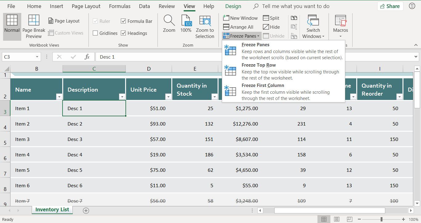
2. Navigate to the View Tab: At the top of the Excel window, locate and click on the "View" tab in the toolbar. This will reveal a set of options related to the visual display of the worksheet.

3. Toggle Gridlines: Within the "View" tab, look for the "Show" group, which contains the "Gridlines" checkbox. By default, this checkbox is selected, indicating that gridlines are visible on the worksheet. To hide the gridlines, simply uncheck the "Gridlines" box. Instantly, the gridlines will disappear from the worksheet, providing a cleaner and more streamlined appearance.

By following these steps, users can easily hide gridlines in Excel using the built-in options, allowing for a more polished and professional presentation of their data. This method provides a quick and convenient way to customize the visual display of a worksheet without altering the actual content or structure of the data.

Hiding gridlines using the Excel options is particularly useful when creating reports, presentations, or documents where a clean and uncluttered appearance is desired. It allows users to focus the viewer's attention on the data itself, rather than the gridlines that delineate the cells.

In addition to enhancing the aesthetic appeal of the spreadsheet, hiding gridlines can also improve the readability and overall impact of the data being presented. Whether for personal use, professional reports, or collaborative projects, mastering this method empowers users to tailor the visual presentation of their Excel worksheets to suit their specific needs and preferences.

Method 2: Using the white font color to hide gridlines

Another clever method to hide gridlines in Excel involves leveraging the font color to effectively mask the gridlines. By strategically adjusting the font color of the cells, users can create the illusion of invisible gridlines, resulting in a clean and polished appearance for their spreadsheets.

To employ this method, follow these steps:

1. Open the Excel Worksheet: Launch Microsoft Excel and open the worksheet from which you want to hide the gridlines.

2. Select the Entire Worksheet: Click on the upper-left corner of the worksheet to select the entire document. This ensures that all cells will be affected by the subsequent formatting changes.

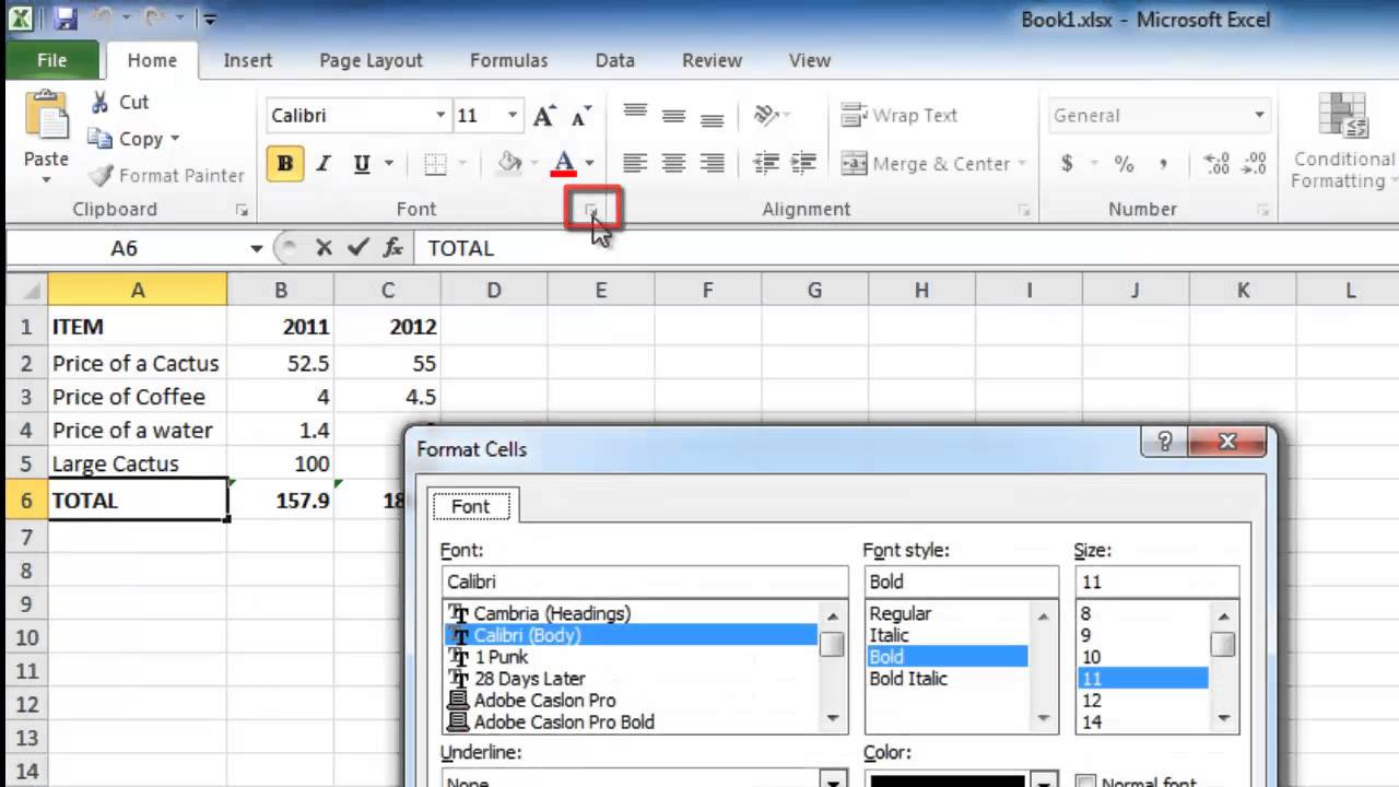
3. Adjust the Font Color: With the entire worksheet selected, navigate to the font color options in the toolbar. Choose the color white as the font color. This effectively makes the text in all cells white, matching the color of the gridlines and creating the illusion that the gridlines have disappeared.

By utilizing the white font color to hide gridlines, users can achieve a seamless and uncluttered appearance for their Excel spreadsheets. This method is particularly effective when the gridlines need to be hidden for presentation or printing purposes, as it allows for a clean and professional look without altering the underlying structure of the data.

Furthermore, this approach offers flexibility, as users can easily revert to the original appearance with visible gridlines by simply changing the font color back to black or any other desired color. This level of control makes it a convenient method for customizing the visual presentation of Excel worksheets based on specific requirements and preferences.

Employing the white font color to hide gridlines is a valuable skill for users who seek to enhance the visual appeal and professionalism of their spreadsheets. Whether for creating reports, financial statements, or data visualizations, mastering this method empowers users to present their data in a visually impactful manner, free from the distraction of visible gridlines.

By incorporating this technique into their Excel proficiency, users can elevate the presentation of their data, ensuring that the focus remains on the content itself, rather than the gridlines that delineate the cells.

Method 3: Adjusting cell borders to hide gridlines

In Microsoft Excel, adjusting cell borders presents a versatile method for concealing gridlines while maintaining the structural integrity of the spreadsheet. This approach allows users to customize the visual presentation of their data without compromising the underlying organization of the cells.

To employ this method effectively, users can follow these steps:

1. Open the Excel Worksheet: Launch Microsoft Excel and open the worksheet from which you want to hide the gridlines.

2. Select the Entire Worksheet: Click on the upper-left corner of the worksheet to select the entire document. This ensures that all cells will be affected by the subsequent formatting changes.

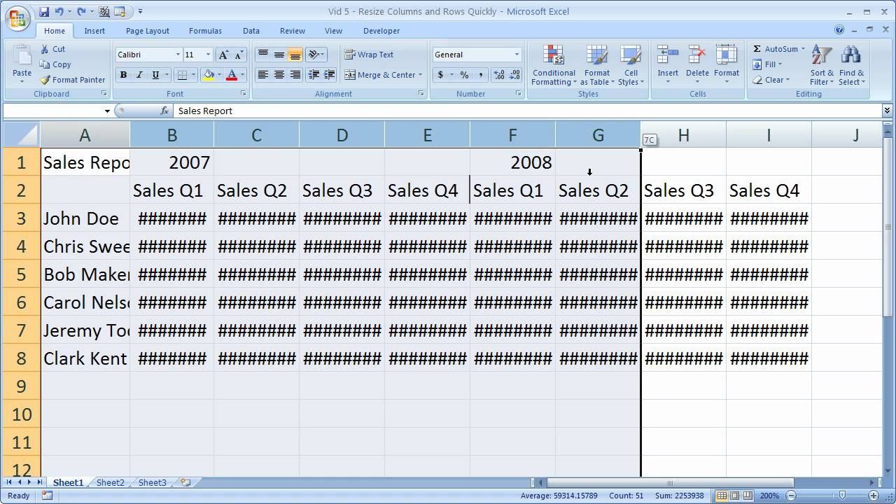
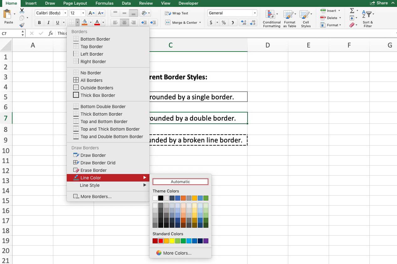
3. Adjust Cell Borders: With the entire worksheet selected, navigate to the "Borders" tool in the toolbar. Here, users can selectively adjust the borders of the cells to effectively hide the gridlines. By removing or modifying specific cell borders, users can create a seamless and uncluttered appearance for their spreadsheets, enhancing readability and visual appeal.

By strategically adjusting cell borders, users can achieve a clean and professional look for their Excel spreadsheets, free from the distraction of visible gridlines. This method is particularly useful when precise control over the visual presentation is desired, as it allows for targeted modifications to the borders of individual cells or cell ranges.

Furthermore, adjusting cell borders to hide gridlines offers a high degree of customization, enabling users to tailor the appearance of their spreadsheets to suit specific requirements and preferences. Whether for financial reports, data analysis, or presentations, mastering this method empowers users to present their data in a visually impactful manner, enhancing the overall clarity and impact of the information being conveyed.

By incorporating this technique into their Excel proficiency, users can elevate the presentation of their data, ensuring that the focus remains on the content itself, rather than the gridlines that delineate the cells. This level of control over the visual presentation of Excel worksheets allows for a polished and professional look, enhancing the overall impact of the data being presented.

Conclusion

In conclusion, the ability to hide gridlines in Microsoft Excel is a valuable skill that empowers users to customize the visual presentation of their spreadsheets, enhancing clarity, professionalism, and overall impact. Throughout this article, we have explored three effective methods for concealing gridlines in Excel, each offering unique advantages and applications.

The first method, utilizing the Excel options to toggle gridlines on and off, provides a quick and convenient way to customize the visual display of a worksheet without altering the actual content or structure of the data. This method is particularly useful for creating reports, presentations, or documents where a clean and uncluttered appearance is desired, allowing users to focus the viewer's attention on the data itself.

The second method, employing the white font color to hide gridlines, offers a clever workaround that creates the illusion of invisible gridlines, resulting in a clean and polished appearance for spreadsheets. This method is especially effective for presentation or printing purposes, as it allows for a professional look without altering the underlying structure of the data, providing flexibility and control over the visual presentation.

The third method, adjusting cell borders to hide gridlines, presents a versatile approach for concealing gridlines while maintaining the structural integrity of the spreadsheet. This method offers precise control over the visual presentation, allowing for targeted modifications to the borders of individual cells or cell ranges, enhancing the overall clarity and impact of the information being conveyed.

By mastering these techniques, users can streamline the visual presentation of their Excel spreadsheets, ensuring that the focus remains on the content itself, rather than the gridlines that delineate the cells. Whether for personal use, professional reports, or collaborative projects, the ability to hide gridlines in Excel is a valuable skill that can significantly improve the overall appearance and impact of the data being presented.

In essence, the methods discussed in this article provide users with the tools to tailor the visual presentation of their Excel worksheets to suit their specific needs and preferences. By incorporating these techniques into their Excel proficiency, users can elevate the presentation of their data, ensuring that the focus remains on the content itself, free from the distraction of visible gridlines.