How To Shade Every Other Row In Excel

(Many of the links in this article redirect to a specific reviewed product. Your purchase of these products through affiliate links helps to generate commission for Noodls.com, at no extra cost. Learn more)

Introduction

Shading every other row in an Excel spreadsheet can significantly enhance the readability and visual appeal of your data. This simple yet effective formatting technique makes it easier for readers to track and compare information across rows, especially in large datasets. Whether you're working on a financial report, inventory list, or any other type of data-driven document, shading alternate rows can make a world of difference in how your information is perceived and understood.

By applying this formatting, you can create a clear visual distinction between rows, reducing the strain on the eyes and helping users focus on specific data points. This technique is particularly useful when presenting data in a tabular format, as it allows for quick and accurate interpretation of the information at hand.

In addition to improving readability, shading every other row can also add a professional touch to your Excel spreadsheets. It demonstrates attention to detail and a commitment to presenting information in a clear and organized manner. Whether you're sharing the spreadsheet with colleagues, clients, or stakeholders, the polished appearance resulting from this formatting choice can leave a positive impression and enhance the overall professionalism of your work.

Moreover, by leveraging Excel's conditional formatting feature to achieve this effect, you can streamline the process and ensure consistency across multiple sheets or workbooks. This means that once you've set up the shading for alternate rows, it will automatically apply to new data added to the spreadsheet, saving you time and effort in the long run.

In the following steps, we'll explore how to shade every other row in Excel using the conditional formatting tool. This straightforward process can be easily mastered by Excel users of all levels, and the results are sure to make a noticeable impact on the visual presentation of your data. Let's dive into the steps to transform your plain spreadsheet into a polished and reader-friendly document.

Step 1: Open the Excel Spreadsheet

Before you can begin shading every other row in Excel, you need to open the spreadsheet containing the data you want to format. Launch Microsoft Excel on your computer and navigate to the location where the spreadsheet is saved. Once you've located the file, double-click on it to open it in Excel.

Upon opening the spreadsheet, take a moment to review the data and identify the specific range of cells that you want to format. This could be a table of sales figures, a list of inventory items, or any other dataset that could benefit from improved readability through row shading.

If you're creating a new spreadsheet from scratch, you can enter your data directly into Excel or import it from another source. Regardless of how the data is populated, the process of shading every other row remains the same.

It's important to ensure that the data is organized in a tabular format, with rows and columns clearly delineated. This will make it easier to select the range of cells for formatting in the subsequent steps. If your data is not yet organized in a tabular layout, take the time to structure it accordingly before proceeding with the shading process.

Once the spreadsheet is open and the data is ready, you're all set to move on to the next step and begin the process of formatting the rows to enhance the visual presentation of your data.

Opening the Excel spreadsheet is the first fundamental step in the process of shading every other row. By familiarizing yourself with the data and ensuring that it is well-organized, you set the stage for a smooth and efficient formatting process. With the spreadsheet open and the data in view, you're ready to proceed to the next step and begin the transformation of your data into a more visually appealing and reader-friendly format.

Step 2: Select the Range of Cells

After opening your Excel spreadsheet and reviewing the data, the next crucial step in shading every other row is to select the range of cells that you want to format. This range will determine which rows receive the alternating shading, so it's essential to choose it accurately.

To select the range of cells, simply click and drag your mouse cursor across the rows that you want to format. You can also click on the first cell in the range, hold down the Shift key, and then click on the last cell to select a contiguous block of cells. Alternatively, if the range is not contiguous, you can hold down the Ctrl key while clicking on individual cells to include them in the selection.

It's important to ensure that the entire range of cells you want to format is included in your selection. This means that all the rows you want to shade should be encompassed within the selected range, and no additional rows should be inadvertently included. Taking a moment to double-check your selection can help prevent errors and ensure that the formatting is applied precisely as intended.

When selecting the range of cells, keep in mind the specific purpose of your data and the audience who will be viewing it. For example, if you're presenting financial data to stakeholders, you may want to format a larger range of cells to ensure that the entire dataset is clearly and consistently formatted. On the other hand, for smaller, more focused tables, a more targeted selection may be appropriate.

By carefully selecting the range of cells, you lay the foundation for a well-organized and visually appealing spreadsheet. This step is crucial in preparing the data for the subsequent formatting actions, ensuring that the shading is applied precisely where it's needed. With the range of cells selected, you're now ready to move on to the next step and delve into the process of applying the alternating row shading to enhance the readability and presentation of your data.

Step 3: Open the Conditional Formatting Menu

To initiate the process of shading every other row in Excel, you need to access the Conditional Formatting menu, which houses a range of formatting options to visually enhance your data. This powerful feature allows you to set rules for formatting cells based on their content, making it an ideal tool for applying alternating row shading.

To open the Conditional Formatting menu, first, ensure that the range of cells you want to format is selected. Once the desired cells are highlighted, navigate to the "Home" tab in the Excel ribbon at the top of the window. Within the "Styles" group, locate and click on the "Conditional Formatting" button. This action will reveal a dropdown menu containing various formatting options.

Upon clicking the "Conditional Formatting" button, a list of formatting rules and options will appear, providing you with the flexibility to choose the most suitable formatting method for your data. In this instance, we will focus on the "New Rule" option, which will allow us to create a custom rule for shading every other row.

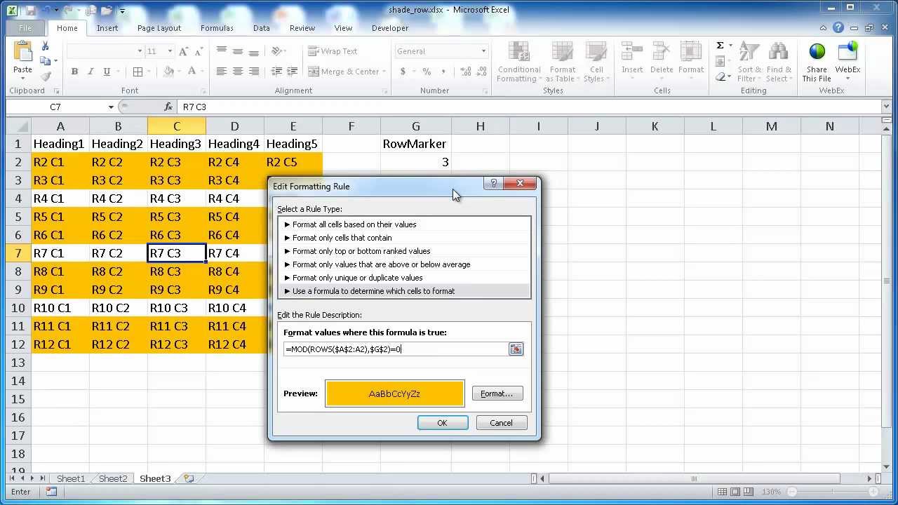
By selecting the "New Rule" option from the Conditional Formatting menu, a dialog box will appear, presenting you with different rule types to choose from. For the purpose of shading every other row, we will opt for the "Use a formula to determine which cells to format" rule type. This selection will enable us to define a formula that specifies the rows to be shaded based on their position within the selected range.

Opening the Conditional Formatting menu marks a pivotal stage in the process of applying alternating row shading to your Excel spreadsheet. This menu serves as the gateway to a myriad of formatting possibilities, empowering you to customize the appearance of your data to suit your specific requirements. With the Conditional Formatting menu now accessible, you are poised to progress to the subsequent steps and delve into the precise configuration of the alternating row shading rule.

Step 4: Choose the Formula Option

Upon selecting the "New Rule" option in the Conditional Formatting menu, you will be presented with a dialog box that offers various rule types to define the formatting criteria. In this step, we will focus on choosing the "Use a formula to determine which cells to format" option, which provides the flexibility to create a custom formula for shading every other row in the selected range.

By opting for the formula option, you gain precise control over the conditional formatting rule, allowing you to specify the exact conditions under which the formatting should be applied. This level of customization ensures that the alternating row shading is tailored to your specific dataset, accommodating varying row counts and content types.

When you choose the formula option, you will encounter a text field where you can input the formula that dictates the formatting rule. The formula you enter will determine the pattern of row shading, instructing Excel to apply the formatting based on the specified conditions. In the case of shading every other row, the formula will target the row numbers and apply the formatting accordingly.

To achieve the alternating row shading effect, the formula should be designed to evaluate the row numbers within the selected range and apply the formatting to alternate rows. Excel provides a simple yet powerful way to accomplish this using the MOD function in conjunction with conditional logic. The MOD function calculates the remainder of a division operation, allowing us to identify even and odd row numbers for the application of formatting.

For example, the formula "=MOD(ROW(),2)=0" can be used to shade every other row starting from the first row in the selected range. Here, the ROW function returns the row number of the cell, and the MOD function checks if the row number divided by 2 yields a remainder of 0, indicating an even row. Based on this evaluation, the formatting will be applied to every other row, creating the desired visual distinction.

By choosing the formula option and crafting a tailored formula to define the shading rule, you harness the full potential of Excel's conditional formatting capabilities. This level of customization empowers you to implement precise and sophisticated formatting rules that align with the unique characteristics of your data, ensuring a professional and polished presentation.

With the formula option selected, you are now equipped to define the specific formula that will govern the alternating row shading, setting the stage for the next steps in the process of enhancing the visual appeal and readability of your Excel spreadsheet.

Step 5: Enter the Formula

After choosing the "Use a formula to determine which cells to format" option in the Conditional Formatting menu, the next pivotal step is to enter the formula that will define the alternating row shading rule. This formula will serve as the guiding logic for Excel to apply the formatting to every other row within the selected range of cells.

To craft the formula, we will leverage the powerful combination of the ROW and MOD functions in Excel. The ROW function returns the row number of a cell, providing us with the essential information to identify the position of each row within the selected range. Meanwhile, the MOD function calculates the remainder of a division operation, allowing us to determine whether a row number is even or odd.

The formula for shading every other row can be succinctly expressed as "=MOD(ROW(),2)=0". Let's break down this formula to understand its functionality:

• ROW(): This function, when used without any arguments, returns the row number of the cell in which it is entered. By employing this function within the conditional formatting formula, we can dynamically obtain the row number for each cell in the selected range.

• MOD(ROW(),2): The MOD function is then applied to the row number obtained from the ROW function. In this context, we divide the row number by 2 and evaluate the remainder. If the remainder is 0, it signifies that the row number is even; otherwise, it is odd.

• =0: The comparison operator "equals 0" is used to check if the result of MOD(ROW(),2) is indeed 0, indicating an even row. When the condition is met, the formula returns TRUE, signifying that the formatting should be applied to the corresponding row.

By entering this formula into the designated text field within the Conditional Formatting dialog box, you instruct Excel to shade every other row based on the calculated conditions. The formula acts as a dynamic rule that adapts to the row numbers within the selected range, ensuring consistent and visually appealing formatting across the spreadsheet.

With the formula accurately entered, you are now ready to proceed to the next step and specify the fill color that will be applied to the alternating rows, bringing your Excel spreadsheet one step closer to a polished and reader-friendly presentation.

Step 6: Choose the Fill Color

With the alternating row shading formula in place, the next crucial step in the process of enhancing your Excel spreadsheet is to choose the fill color that will be applied to the formatted rows. This step allows you to customize the visual appearance of the shaded rows, aligning the formatting with your preferred color scheme or design aesthetic.

Upon entering the formula for alternating row shading and confirming it within the Conditional Formatting dialog box, you will encounter an option to specify the fill color for the formatted cells. This presents an opportunity to infuse your spreadsheet with a touch of personalization and visual appeal, elevating the overall presentation of your data.

When choosing the fill color, it's important to consider the readability and visual contrast of the shaded rows. Opting for a color that distinctly stands out against the default cell color while maintaining legibility is essential. Additionally, the chosen fill color should complement the overall design of your spreadsheet and align with any existing color schemes or branding guidelines.

Excel offers a wide range of fill color options, allowing you to select from a palette of standard colors or create custom shades to suit your preferences. Whether you prefer a subtle, muted tone for the shaded rows or a bold, vibrant color to make a striking visual impact, Excel's formatting tools provide the flexibility to achieve your desired aesthetic.

Furthermore, the choice of fill color can also convey specific meanings or highlight particular types of data within your spreadsheet. For example, you may opt for a light green fill color to signify positive values or achievements, while a light red shade could be used to draw attention to areas requiring further review or action.

By carefully selecting the fill color for the shaded rows, you add a layer of visual distinction and organization to your data, enhancing the overall readability and impact of the spreadsheet. This attention to detail demonstrates a commitment to presenting information in a clear and visually engaging manner, leaving a positive impression on those who interact with your data.

With the fill color chosen, you are now poised to apply the formatting and witness the transformation of your Excel spreadsheet into a polished and reader-friendly document, where the alternating row shading enhances the visual appeal and accessibility of your data.

Step 7: Apply the Formatting

After defining the alternating row shading formula and selecting the fill color, the final step in the process of enhancing your Excel spreadsheet is to apply the formatting to the selected range of cells. This pivotal action brings the visual transformation to life, imbuing your data with a professional and polished presentation that is sure to captivate and engage your audience.

To apply the formatting, simply click the "OK" button within the Conditional Formatting dialog box. This action confirms the custom rule you've defined and instructs Excel to implement the alternating row shading based on the specified formula and fill color. Upon clicking "OK," you will witness the immediate application of the formatting to the selected range, with every other row now adorned with the designated fill color.

As the formatting is applied, take a moment to observe the visual impact it has on your data. The alternating row shading creates a clear and organized layout, making it easier for readers to track and compare information across rows. The distinct visual separation between rows reduces eye strain and enhances the overall readability of the spreadsheet, ensuring that your data is presented in a manner that is both professional and accessible.

Furthermore, the application of the formatting demonstrates your attention to detail and commitment to presenting information in a visually engaging manner. The polished appearance resulting from the alternating row shading showcases your dedication to delivering clear and organized data, leaving a positive impression on those who interact with your spreadsheet.

It's important to note that once the formatting is applied, it will automatically adapt to any changes made within the selected range. Whether you add new data, modify existing entries, or expand the range of cells, the alternating row shading will seamlessly adjust to maintain the visual distinction across rows. This ensures consistency and efficiency in presenting your data, saving you time and effort in managing the spreadsheet's visual formatting.

With the formatting successfully applied, you have transformed your Excel spreadsheet into a visually appealing and reader-friendly document. The alternating row shading serves as a testament to your commitment to presenting data in a clear and organized manner, setting the stage for enhanced interpretation and understanding of the information at hand.

Conclusion

In conclusion, the process of shading every other row in Excel using conditional formatting offers a straightforward yet impactful method to enhance the visual presentation and readability of your data. By following the step-by-step guide outlined above, you can transform a plain and utilitarian spreadsheet into a polished and reader-friendly document that captivates and engages your audience.

The application of alternating row shading serves as a visual aid, allowing readers to track and compare information across rows with ease. This simple formatting technique reduces eye strain and enhances the overall readability of the data, making it particularly valuable when presenting large datasets or tabular information. The distinct visual separation between rows creates a clear and organized layout, ensuring that your data is presented in a manner that is both professional and accessible.

Furthermore, the customization options offered by Excel's conditional formatting feature enable you to tailor the shading to suit your specific design preferences and data requirements. From choosing the fill color to crafting a formula that precisely defines the shading rule, you have the flexibility to align the formatting with your preferred color scheme or branding guidelines, adding a touch of personalization to your spreadsheet.

The attention to detail demonstrated through the application of alternating row shading reflects a commitment to presenting information in a visually engaging manner. This level of care and precision leaves a positive impression on those who interact with your data, showcasing your dedication to delivering clear and organized information.

Moreover, the dynamic nature of the formatting ensures that it seamlessly adapts to changes within the selected range of cells, maintaining consistency and efficiency in presenting your data. Whether you're adding new data, modifying existing entries, or expanding the range, the alternating row shading will adjust accordingly, saving you time and effort in managing the visual formatting of your spreadsheet.

In essence, the process of shading every other row in Excel using conditional formatting empowers you to elevate the visual appeal and accessibility of your data, making a significant impact on how your information is perceived and understood. By leveraging this simple yet powerful formatting technique, you can create a professional and polished spreadsheet that effectively communicates your data while leaving a lasting impression on your audience.